ACEMS 2017 Student "Sampling & Exploration Competition"

Congratulations to our 2017 Winners!

matlab-winners.jpg

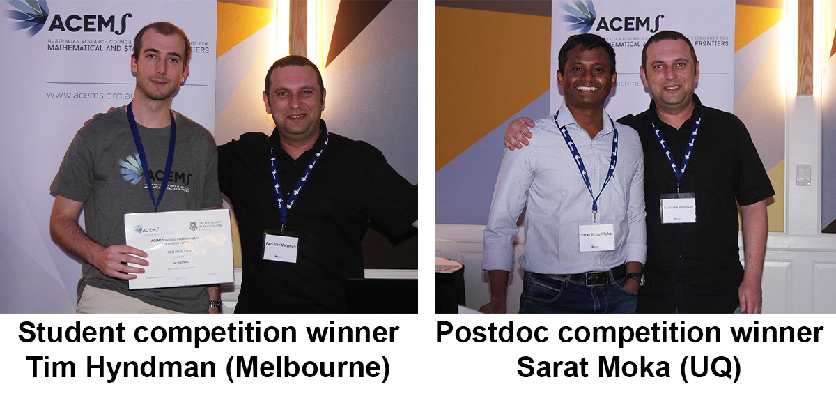
The winners of the 2017 competition were Tim Hyndman (The University of Melbourne) and Sarat Moka (The University of Queensland). Both are pictured above with Slava Vaisman (UQ), one of the two organisers of the competition. The other organiser was Prof Dirk Kroese (UQ).

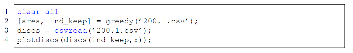
Final Results

Student Competition

1. Tim Hyndman, The University of Melbourne
2. Jun Chen, UNSW
3. Krzysztof Bisewski and Nick Verheul, Centrum Voor Wiskunde en Informatica

Postdoc Competition

1. Dr Sarat Moka, The University of Queensland
2. Dr Wilson Chen, UTS

Competition details:

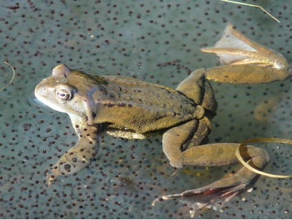
frida-frog.jpg

Figure 1 - Frida Frog

Advanced Sampling and Exploration Mathematics Competition, 2017

Dirk P. Kroese and Slava Vaisman

School of Mathematics and Physics

The University of Queensland, Australia

In an article in the Notices of the American Mathematical Society, Freeman Dyson divides mathematicians into two types: Birds and Frogs. Birds fly high in the air and survey broad vistas of mathematics, delighting in concepts that bring together diverse problems from different parts of the landscape. Frogs live in the mud below and see only the flowers that grow nearby, cherishing the details of particular objects, and solving problems one at a time.

Whether you are a Bird or a Frog, spare a thought for the plight of Frida Frog, who "ponders" the following problem. She has laid too many of her eggs on a flat torus (a square with wrapped-around borders) and would like to thin them out such that none of the eggs overlap. However, all of the remaining eggs should keep their current positions. Viewing her eggs as two-dimensional disks, she would like the total area of the remaining eggs to be as large as possible.

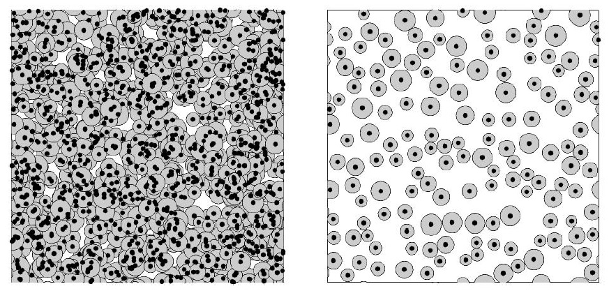
disks-competition.jpg

Figure 2: Discs unthinned (left) are thinned out (right) such that no two discs overlap. Discs that intersect the borders wrap around to the opposite side.

1.  The Problem

Frida's eggs can be considered to be perfect discs, not necessarily of the same radius. Before thinning, there are N disks, whose centres are uniformly and randomly distributed over the unit square. After thinning, none of the remaining discs intersect and all retain their original positions and radii. The situation is illustrated in Figure 2. Note that the problem - which set of non-overlapping discs to select in order to obtain the maximal area - is completely determined by the centres and radii of the N original discs. This information will be stored in a CSV (comma separated values) file with N rows and 3 columns. The first two columns give the x- and y-coordinates of the disc centres, and the third column gives the radii of the discs.

The challenge is to determine, for various scenarios, which discs should be retained so as to maximize the total area covered by the retained discs.

2. The Competition

The competition is open to all students. Submissions are accepted from individuals and teams. The winning entry will receive a $1200 award. Second and third place receive $600 and $200, respectively, The deadline for submissions is 3 October, 2017 (23:59:59, UTC-12). Winners will be announced at the ACEMS retreat, from 31 October to 3 November, 2017. Please send your submission to slvaisman@gmail.com with a copy to kroese@maths.uq.edu.au.

• CLICK HERE to access lead tables, data sets, and accompanying Matlab code 

The objective is to find the optimal solution for each of 11 scenarios. For eight of these scenarios the corresponding CSV data sets are known. For the other three scenarios the data sets remains hidden.

Table 1 provides details about the eight known scenarios. The second column gives the names of the data sets, the third column shows how the radii were generated, and the fourth column provides the available scores (details on the scoring are given later).

The first number in the name of the data set specifies the number of discs. For example, data set 1000.1.csv has N = 1000 discs. In five cases the radii are fixed (scenarios 1, 3, 5, 7, 8). In scenarios 2 and 4 the radii are independently and uniformly drawn from intervals (0.02, 0.04) and (0.02, 0.07), respectively. In scenario 6 the radii are drawn independently from a two-point distribution, taking values 0.01 and 0.1 with probability 1/2 each.

• Table 1: Information for the eight known scenarios.

table1.png

For the eight known scenarios it suffces to submit only a list of indices of the discs that are remaining (the ones that are not thinned out). Provide such lists in CSV format. For an input file 200.1.csv, name the submitted output file TeamName.200.1.csv, where TeamName is the name of your team. You may use any program, C++, R, Matlab, Python, Java, etc., to construct such a list. If you wish to enter the competition for the three unknown scenarios, you must submit a Matlab function that takes the CSV input file as its sole argument and outputs the area and a column vector with the indices of the "remaining" discs. This program, whose name should again start with the name of your team, should be able to distinguish between the different scenarios via the name of the input le. For example, 500.2.hidden.csv might need a different solution strategy than 1000.1.hidden.csv.

The program may run for a maximum of 15 minutes on each of the 3 hidden scenarios, using our local computer (45 minutes in total). You may use fix(clock) to check if your time is running out.

The current largest known values (areas) for all 11 scenarios will be listed on the website given above, and updated when any better solution is found. You may provide solutions to all or a selection of the 11 scenarios, but you may only submit a maximum of three times times during the competition.

We reserve the right to modify the time limits and maximal number of submissions, if it is not possible to process all submissions in time. These modifications will be announced on this web page.

As mentioned, the lead table will maintain a list of the largest values (areas) found so far, for all 11 scenarios. It also lists the next two entries for each scenario. For a scenario with maximal available score s (given in Table 1 and a score of 5 for each hidden scenario), the best entry receives a score of 2/3 × s, the next best entry receives 2/9 × s, and the third best entry 1/9 × s. The maximal total score for any team is thus 2/3 × 45 = 30.

Prizes will be awarded based on the ranking of the total scores at the close of the competition. If at any time two submissions are received that report the same maximum value (but with a different list of indices), the one that was received earlier is ranked higher than the later entry.

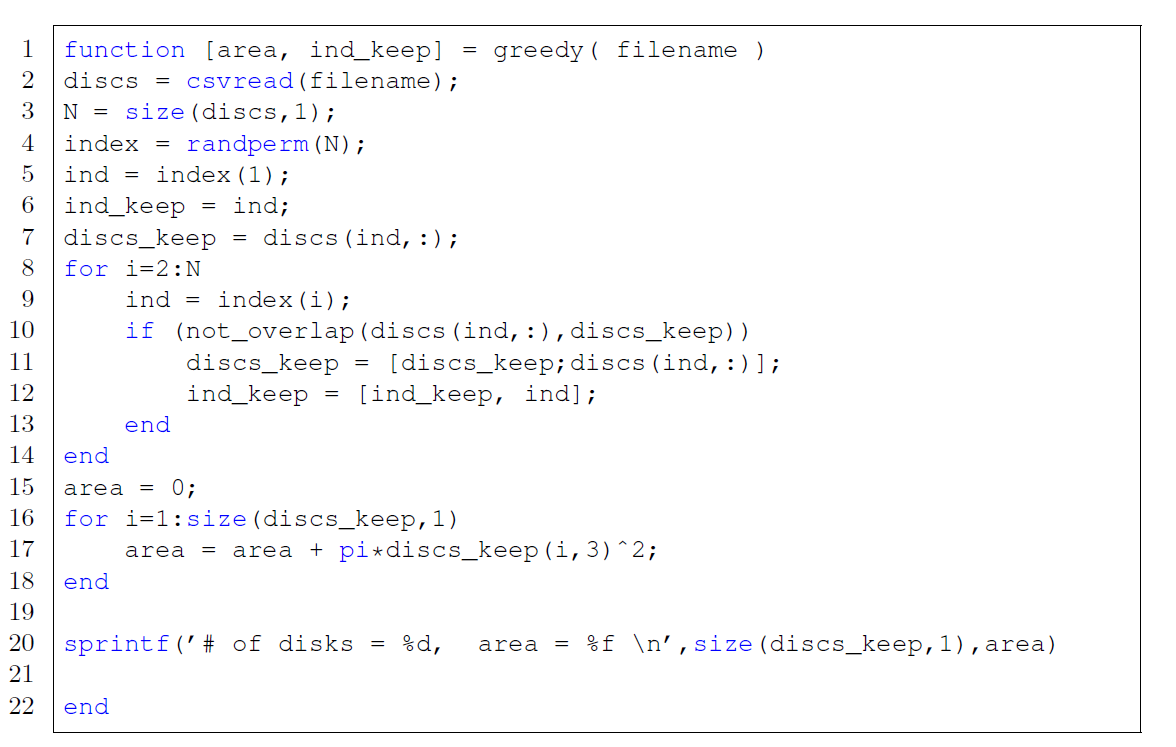
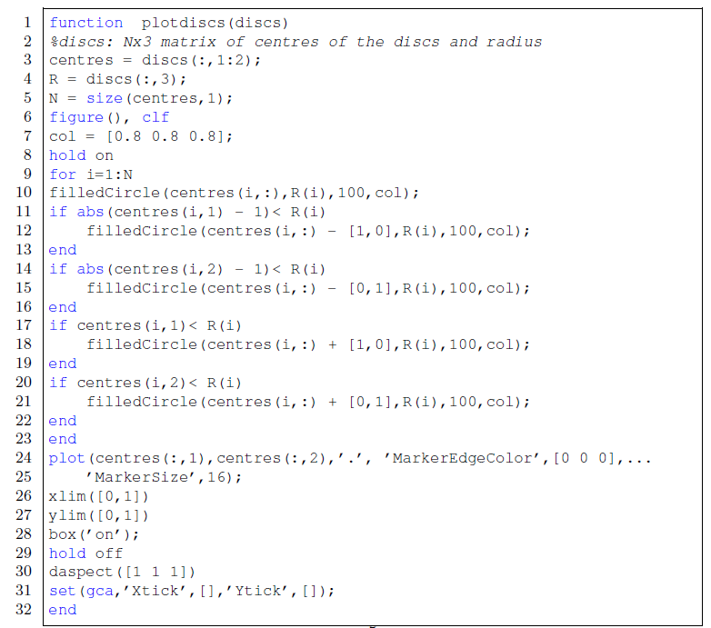
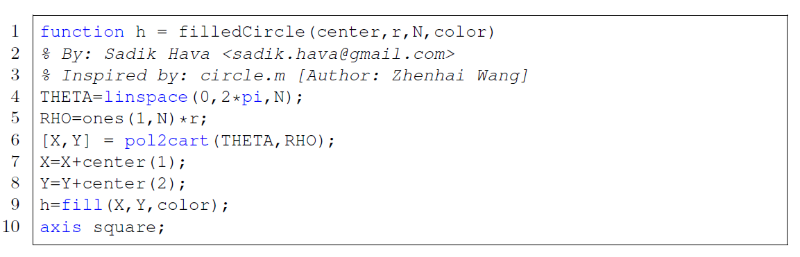
5. Example Code

Below is some Matlab code that may help you on your way. The first function implements a greedy strategy, where new discs are chosen in random order and added to a list of retained discs if they do not overlap with any of the previously chosen ones. It uses the function not overlap, given below, to check if a disc overlaps with any of a given set of discs.

code1.png

table2.png

Here is an example of a script to run in the greedy algorithm.

table-3.png

The function plotdiscs plots the discs, which are "wrapped over" to the other side if they intersect the boundaries of the unit square.

table-4.png

table-5.png

Finally, Table 2 shows the results from one run of the greedy algorithm. There is still a lot of improvement possible. For example, Figure 3 shows the remaining discs obtained via the greedy algorithm for the 50000.1.csv data set. As there are 50000 discs centres to choose from, uniformly spread over the torus, it is clear that the discs should be able to be packed much closer, in a close to hexagonal pattern.

• Table 2: Results from one run of the greedy algorithm.

table-2.png

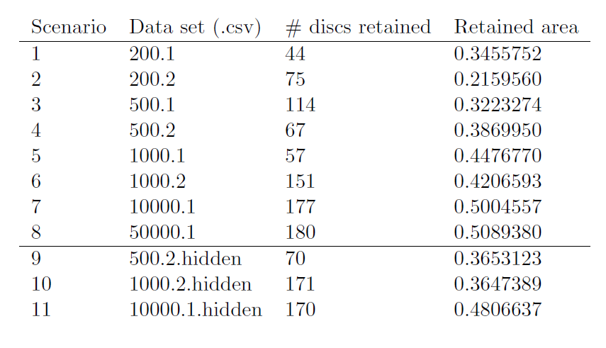
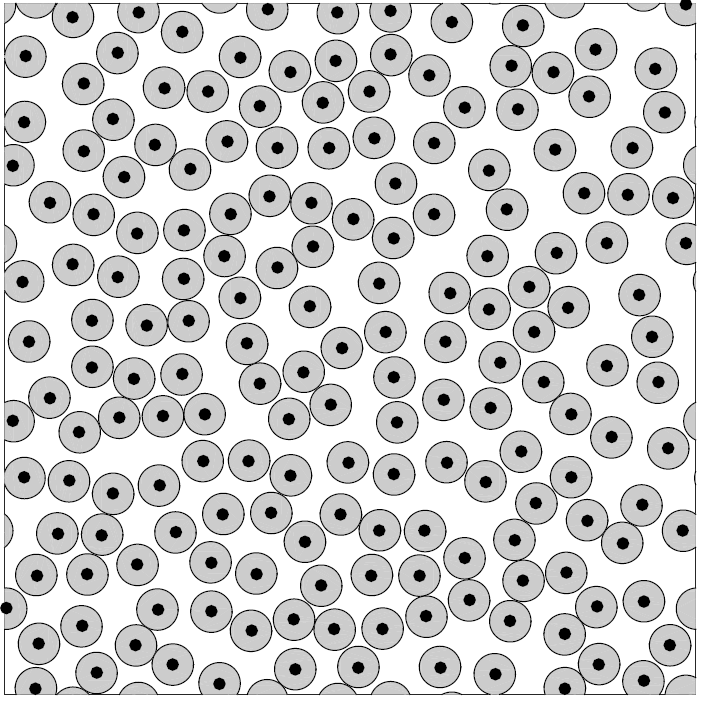
figure3.png

Figure 3: Remaining discs for 50000.1.cvs. The complete set of 50000 possible disc centres have not been plotted, but it should be clear that the discs can be packed much closer.